SAN: Location Optimizer

1. Abstract
2. Nodes
3. Genetic algorithm for location optimization
4. Simulation
5. Experimentation
6. Examples

1 Abstract

The location optimizer takes all the data that is available and guesses the locations of the nodes in space.

Input:

which node is connected to which node and on which port,
tilt angles of nodes (optional).

Output:

locations of the nodes in space,
tilt angle of spheres for display (optional).

The location optimizer does its calculations under the assumption that:

the length of a connection is 1,
the angle between connections is the tetrahedral angle (≈ 109.5°).

Note that the information in this document is only relevant for the version of SAN that was current at the time of publication.

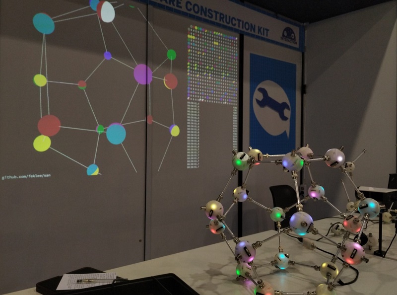
Figure 1: Dodecahedron built by two little girls at the end of Maker Faire Rome: Convergence successful!

2 Nodes

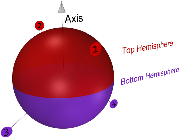
Figure 2: Geometry of a node with ports 1–4

Properties of a node:

A node may also be called a sphere, referring to the physical elements in the SAN construction kit.
There is one special node, the root node:
- It connects the computer to the network.
- It has one USB port that connects to the computer.
- It has only one port: 1
- It’s ID is: ^
Non-root nodes have four ports: 1, 2, 3, and 4
Each non-root node has a unique ID: A–Z
A node’s axis is relevant if there is information about its tilt angle. The tilt angle is measured by an accelerometer. As of this writing there is only one sphere that contains an accelerometer.

3 Genetic algorithm for location optimization

3.1 Summary

A genetic algorithm is used to approximate the positions of the points in space. This algorithm is called location optimizer. After optimization, ideally all neighboring nodes have a distance of 1, and the angles between the connecting edges match those on the spheres. The algorithm, however, is flexible enough to find solutions even if distances or angles have been violated. See examples below.

3.2 Steps

Initialize: Generate a population of $n$ individuals. Each individual $i$ is described by a chromosome $X_i$. A chromosome contains a list of coordinates. The coordinates describe a distribution of points in space. Initially the coordinates are chosen randomly.

Example population for a network composed of nodes $C$, $B$, and $D$:

	$x_C$	$y_C$	$z_C$	$x_B$	$y_B$	$z_B$	$x_D$	$y_D$	$z_D$
$X_1$	-0.87	-0.59	0.51	0.01	-0.18	0.92	-0.88	-0.45	-0.61
$X_2$	0.14	0.39	0.37	0.30	-0.61	-0.25	0.40	0.21	0.75
$X_3$	0.40	-0.54	0.00	-0.43	0.94	0.29	0.37	0.76	-0.74
…
$X_n$	0.08	-1.00	0.71	-0.68	-0.26	0.33	-0.64	0.94	0.95

Reproduce:
1. Pair: Randomly select pairs of individuals. These individuals will act as parents in the next step.
  
  Example pair: $(X_3, X_1)$
2. Create offspring. For each pair of parents:
  1. Crossover: Form a child chromosome by taking one part of the chromosome from the first parent and the other part from the second parent.
    
    Child created from a crossover of the above example pair:
    
    $X_3$: $x_C$ … $x_D$ $X_1$: $y_D$ … $z_D$
    
    0.40 -0.54 0.00 -0.43 0.94 0.29 0.37 -0.45 -0.61
    
    The location of the crossover is random. More than one crossover may happen, i.e. switching multiple times from the chromosome of one parent to that of the other.
  2. Mutate: Randomly change coordinates in the child chromosome.
    
    Example mutation of the above child:
    
    0.40 -0.54 -1.50 -0.43 0.94 0.29 0.37 -0.45 0.40
Find fitness: For each child determine how close the coordinates in the chromosome are to an optimal distribution. An optimal distribution is one where:
- the distance between each two neighboring nodes is 1,
- the angle between each two connections from one node is the tetrahedral angle.
The deviation to the optimal distribution is quantified as fitness and assigned to each child.
Natural selection: Create a new population by combining:
- the $n - 1$ best children,
- the best individual from the previous generation.
Visualization: Render the best individual in the new population on screen.
Iterate: go to step 2.

\(X_3\): \(x_C\) … \(x_D\)	\(X_1\): \(y_D\) … \(z_D\)
0.40 -0.54 0.00 -0.43 0.94 0.29 0.37	-0.45 -0.61

3.3 Problem

Genetic algorithms tend to get stuck in local minima. In that case all individuals have converged close to the same non-optimal solution. Mutation of single coordinates worsen the fitness of an individual. Therefore, differing individuals don’t carry over to the next generation. Evolution has stopped.

3.4 Fitness

Fitness is a measure for the deviation from the optimum. But how do we calculate the deviation if we don’t know the optimum? Let’s see!

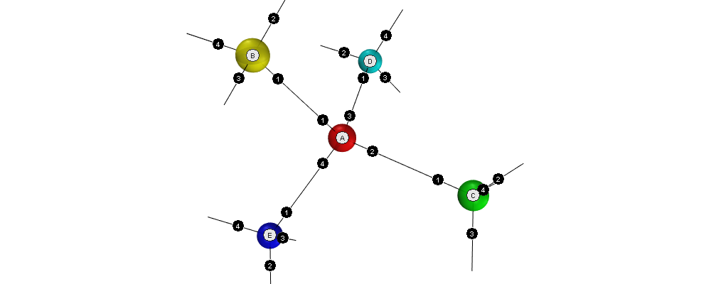
The idea is to calculate the deviation from the optimum for each node, then sum all deviations. What follows is an example for node $A$ with a full set of neighbors, $B$, $C$, $D$, and $E$.

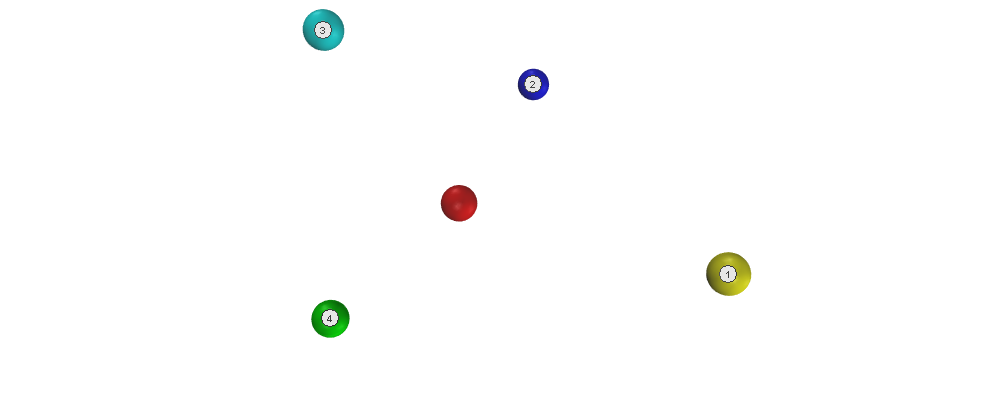
In this example, the connections for node $A$ are:

Connection 1: port 4 connected to node $B$ (yellow)
Connection 2: port 1 connected to node $E$ (blue)
Connection 3: port 3 connected to node $D$ (aqua)
Connection 4: port 2 connected to node $C$ (lime)

3.4.1 Deviation of first neighbor

Correct neighbor locations lie on a sphere of radius 1. As the location of the expected neighbor $1'$, we take the point that is closest to the location of the existing neighbor $1$ (deviation highlighted in red):

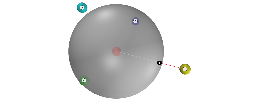
The deviation is the difference between the two locations:

$D_{A,1} = 0.50$

3.4.2 Deviation of second neighbor

Correct neighbor locations are at the tedrahedral angle to the edge connecting the node and its first expected neighbor $1'$. In addition, correct neighbor locations are required to have a distance of 1 from the center. Therefore, the set of all correct locations lies on a circle. As the location of the expected neighbor $2'$ we select from this set the point that is closest to the exising neighbor $2$.

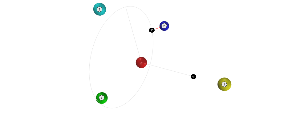
Deviation:

$D_{A,2} = 0.28$

3.4.3 Deviations of third and fourth neighbor

Based on the locations of the first two expected neighbors $1'$ and $2'$, we can calculate the locations of the remaining expected neighbors $3'$ and $4'$.

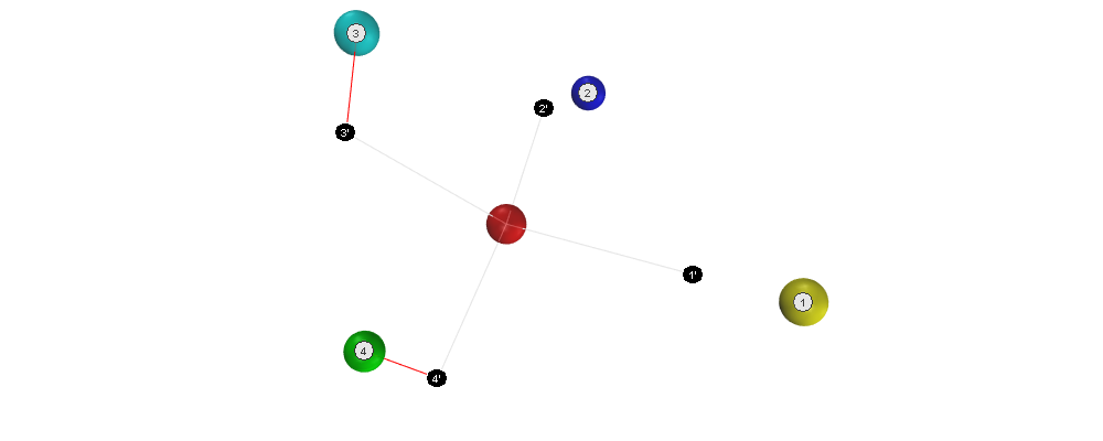
Deviations:

$D_{A,3} = 0.49, D_{A,4} = 0.63$

3.4.4 Total deviation

Now we can calculate the total deviation of all the neighbors of the node:

$D_A = D_{A,1} + D_{A,2} + D_{A,3} + D_{A,4} = 1.90$

After the deviation has been calculated for every node, the total deviation can be calculated. For a network with nodes $A$, $B$, $C$, $D$, and $E$ that would be:

$D = D_A + D_B + D_C + D_D + D_E$

To get the fitness $F$ of the current chromosome, we simply reverse the sign:

$F = -D$

As the value of the deviations is negative, it holds that: The higher the fitness, the closer the individual is to an optimal solution.

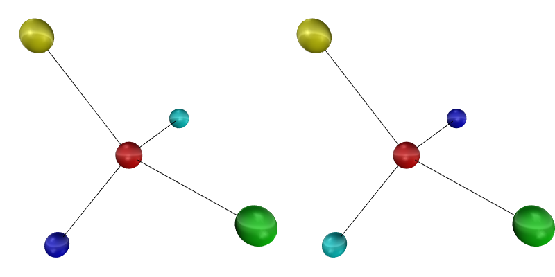
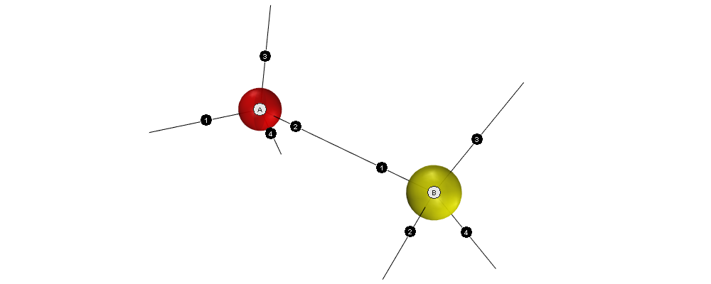
3.4.5 Note about the positions of the third and fourth neighbor

Note that for calculating the positions of connections 3 and 4, the position of the ports is relevant. Take a look at the following two structures. They are not identical!

3.5 Alternative fitness proposal

The following proposal creates the fitness based on the sum of independent terms. The terms may possibly be multiplied by weights. With the first two terms, this fitness has been used as cost function in David’s San-Optimizer based on the gradient descend algorithm. Another suggestion is to use the conjugate gradient method.

3.5.1 Distance

\begin{equation} F_D = \sum_{n=1}^N (l_n^2 - 1)^2 \end{equation}

Where:

$N$: number of all edges
$l_n$: length of edge $n$

$1$ is the expected distance.

3.5.2 Angle

\begin{equation} F_A = \sum_{n=1}^N \sum_{i=1}^{I_n} \sum_{j=1\\j≠i}^{I_n} (\vec{v}_{n,i} ⋅ \vec{v}_{n,j} + ⅓)^2 \end{equation}

Where:

$N$: number of nodes
$I_n$: number of neighbors attached to node number $n$
$v_{n,i}$: vector connecting node number $n$ to neighbor number $i$

$-⅓$ is the cosine of the required tedrahedral angle.

Note that the vectors are not normalized. Nevertheless optimization works in David’s implementation.

3.5.3 Chirality

\begin{equation} F_C = \sum_{n=1}^L \Big((\vec{v}_{n,1}^L × \vec{v}_{n,2}^L) ⋅ \vec{v}_{n,3}^L - cos\big(\frac{π}{2} - \frac{1}{2} arccos(-⅓)\big)\Big)^2 + \\ \sum_{n=1}^R \Big((\vec{v}_{n,1}^R × \vec{v}_{n,2}^R) ⋅ \vec{v}_{n,3}^R - cos\big(\frac{π}{2} + \frac{1}{2} arccos(-⅓)\big)\Big)^2 \end{equation}

Where:

$L$: number of nodes with left handed chirality
$R$: number of nodes with right handed chirality
$v_{n,i}^{L/R}$: normalized vector connecting left/right handed node number $n$ to its neighbor number $i$

Only nodes with at least three neighbors are included. The other nodes don’t have chirality.

3.5.4 Tilt

Some nodes provide tilt information by means of an accelerometer, the tilt angle $α$. Tilt is measured against the z-axis $\vec{z}$. To work with tilt, we introduce an additional unknown, the tilt axis $\vec{a}_n$. For node number $n$ we get the term:

\begin{equation} F_{T,n} = (\vec{z} ⋅ \vec{a}_n - cos(α)) \end{equation}

For visualization, the colored hemispheres of a node are oriented along the tilt axis.

3.5.5 Orientation

With tilt, there is a constraint on the orientation of connections. Relative to the tilt axis, connections on ports 1 and 2 are oriented at half tetrahedral angle $τ$ whereas connections on ports 3 and 4 are oriented at $π/2 - τ$. The fitness term is $F_O$.

3.5.6 Total fitness

The total fitness is:

\begin{equation} F = -(w_D F_D + w_A F_A + w_C F_C + w_T F_T + w_O F_O) \end{equation}

Where $w_i$ are weights.

4 Simulation

Assembling the structure can be simulated. This is useful for testing the location optimizer without the physical construction kit.

Setup:

Install Node.js and the Yarn package manager.
Clone the SAN repository from: https://github.com/feklee/san/
Install all necessary dependencies and build the frontend (on Windows call rollup.cmd instead of rollup):
```
$ cd webapp
$ yarn install
$ ./node_modules/.bin/rollup --config
```
Start the simulation:
```
yarn start simulate
```
Open the SAN web app: http://localhost:8080

To navigate in 3D in the canvas on the left side, use the mouse.
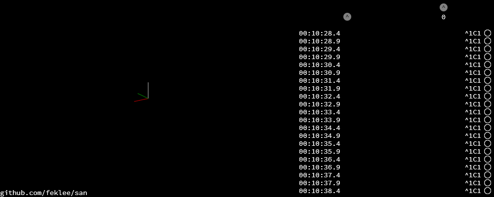
Go back to the command line and connect a node to the root node:
```
+^1C1
```
This connects port C1 (port 1 on node C) with ^1 (port 1 on the root node). The result is immediately visible in the web app.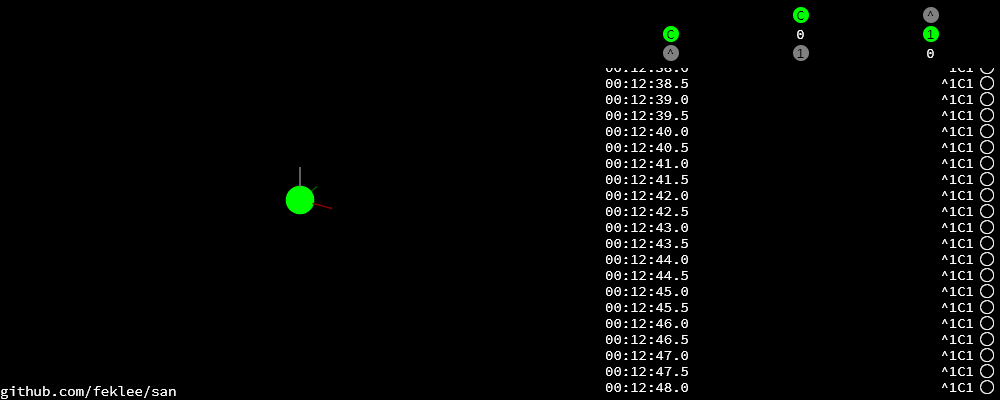

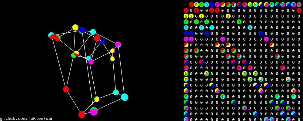
On the top right side you see an adjacency matrix. The numbers in the matrix refer to the connected ports. On the bottom right side you see a log of the information that the webapp receives from the structure. Each line begins with a timestamp. The circle on the right means that there is no information about a tilt angle for the connected node.
Add additional nodes:
```
+C2B1
+B3D4
```
This connects B3 (port 3 on node B) to C2 and D4 to B3.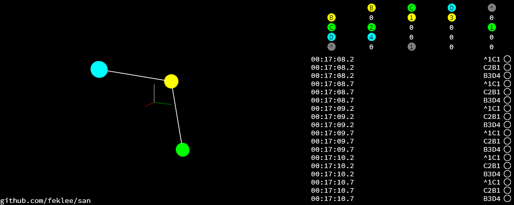

5 Experimentation

For experimentation, custom locations may be assigned to nodes.

Open the SAN web app.
Make sure that you see the network that you want to work with.
Open your browser’s JavaScript console.
Stop the location optimizer:
```
locationOptimizer.stop();
```

Assign the locations, for example:

locationOptimizer.setLocations({
    A: [0, 0, 0],
    B: [1, 0, 0],
    C: [1, 1, 0],
    D: [0, 1, 0]
});

Optionally, update the locations in the location optimizer and resume optimization:
```
locationOptimizer.update();
locationOptimizer.run();
```
Caution: If your locations cannot compete with the locations in the current population, you will not see them in the next generation. They will disappear immediately.

6 Examples

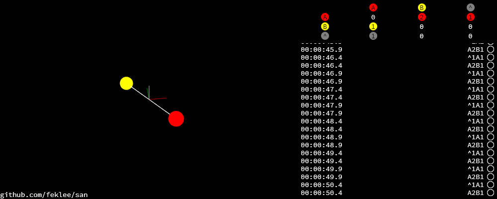
6.1 1:1

Just two nodes are connected.

6.1.1 Input

Simulation:

+^1A1
+A2B1

Adjacency matrix (numbers are ports): 1-1-adjacency.tsv

6.1.2 Example solution

Coordinates: 1-1-coordinates.tsv

6.2 1:4

One node has all of its four neighbors connected.

6.2.1 Input

Simulation:

+^1B2
+B1A1
+A2C1
+A3D1
+A4E1

Adjacency matrix (numbers are ports): 1-4-adjacency.tsv

6.2.2 Example solution

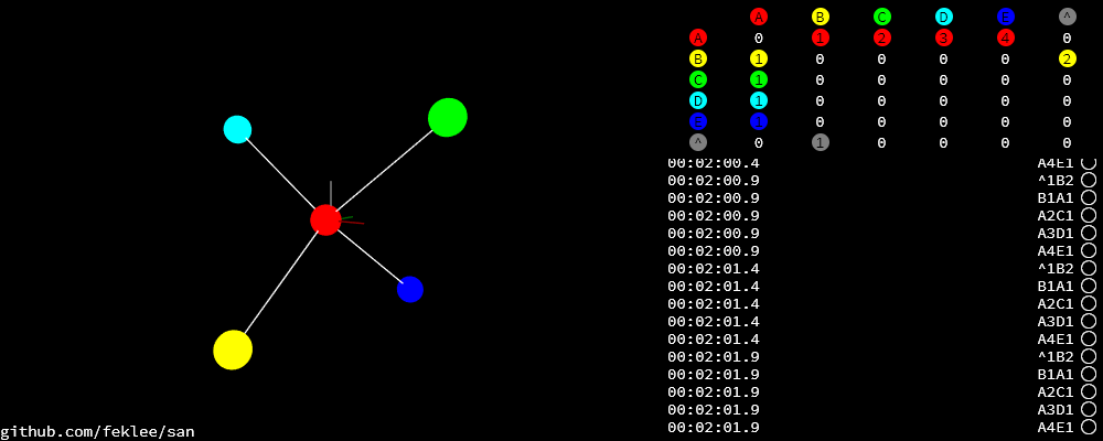
Coordinates: 1-4-coordinates.tsv

6.3 Hexagon

This is the smallest loop that can be built without violating the tetrahedral angles.

6.3.1 Input

Simulation:

+^1A1
+A2B1
+B2C1
+C2D1
+D2E1
+E2F1
+F2A3

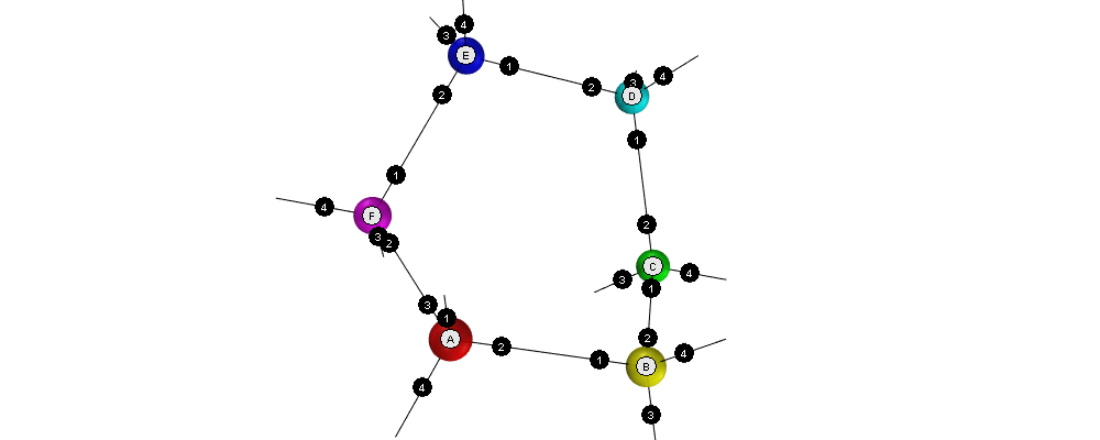
Adjacency matrix (numbers are ports): hexagon-adjacency.tsv

6.3.2 Example solution

Coordinates: hexagon-coordinates.tsv

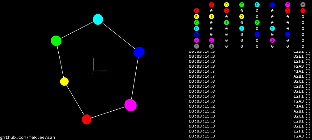
6.4 Pentagon

Note that the interior angles of a pentagon are 108°. That is close to but not identical to the tetrahedral angle of 109.5°. Nevertheless the algorithm is able to approximate a solution. Even for nodes connected in a triangle it finds a solution!

6.4.1 Input

Simulation:

+^1A1
+A2B1
+B2C1
+C2D1
+D2E1
+E2A3

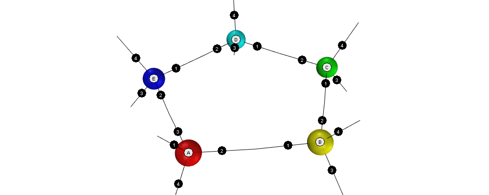
Adjacency matrix (numbers are ports): pentagon-adjacency.tsv

6.4.2 Example solution

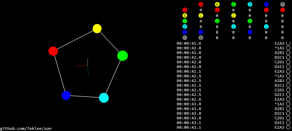
Coordinates: pentagon-coordinates.tsv

6.5 Dodecahedron

The dodecahedron consists of twelve pentagon sufaces. There are 20 unknown edges, i.e. nodes in the network. This means 60 variables have to be found.

6.5.1 Input

Simulation:

+^1A4
+A1B2
+A2E1
+A3F1
+B1C2
+B3H1
+C1D2
+C3J1
+D1E2
+D3L1
+E3N1
+F2O2
+F3G3
+G1P1
+G2H2
+H3I3
+I1Q1
+I2J2
+J3K3
+K1R1
+K2L2
+L3M3
+M1S1
+M2N2
+N3O3
+O1T1
+P2T3
+P3Q2
+Q3R2
+R3S2
+S3T2

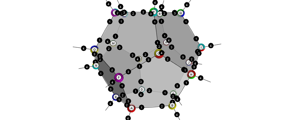
Adjacency matrix (numbers are ports): dodecahedron-adjacency.tsv

6.5.2 Example solution

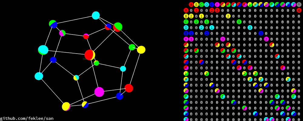
Coordinates: dodecahedron-coordinates.tsv

6.5.3 Example bad solution

In most runs, at least nine out of ten times, the genetic algorithm does not find a good solution. It gets stuck in a local minimum.

6.6 Dodecahedron with tilt angles

Tilt angles provide additional information. The idea is to reduce the space of unknown variables from 60 to 40, thereby making it easier to find a solution. On the other hand, calculation of fitness is more cumbersome and, at least in the current implementation, more time consuming.

Results have been mixed. In fact it looks like convergence now is almost unachievable.

Another purpose for tilt information is to get a more accurate represantation of what the user actually built. Without tilt information, for example, the displayed structure may be upside down compared to what the user sees sitting on the table.

6.6.1 Input

Simulation (/A92 sets the tilt angle of node $A$ to 92°):

+^1A4
+A1B2
+A2E1
+A3F1
+B1C2
+B3H1
+C1D2
+C3J1
+D1E2
+D3L1
+E3N1
+F2O2
+F3G3
+G1P1
+G2H2
+H3I3
+I1Q1
+I2J2
+J3K3
+K1R1
+K2L2
+L3M3
+M1S1
+M2N2
+N3O3
+O1T1
+P2T3
+P3Q2
+Q3R2
+R3S2
+S3T2
/A92
/B92
/C92
/D92
/E92
/F107
/G73
/H107
/I73
/J107
/K73
/L107
/M73
/N107
/O73
/P135
/Q135
/R135
/S135
/T135

	\(x_C\)	\(y_C\)	\(z_C\)	\(x_B\)	\(y_B\)	\(z_B\)	\(x_D\)	\(y_D\)	\(z_D\)
\(X_1\)	-0.87	-0.59	0.51	0.01	-0.18	0.92	-0.88	-0.45	-0.61
\(X_2\)	0.14	0.39	0.37	0.30	-0.61	-0.25	0.40	0.21	0.75
\(X_3\)	0.40	-0.54	0.00	-0.43	0.94	0.29	0.37	0.76	-0.74
…
\(X_n\)	0.08	-1.00	0.71	-0.68	-0.26	0.33	-0.64	0.94	0.95

SAN: Location Optimizer

Table of Contents

1 Abstract

2 Nodes

3 Genetic algorithm for location optimization

3.1 Summary

3.2 Steps

3.3 Problem

3.4 Fitness

3.4.1 Deviation of first neighbor

3.4.2 Deviation of second neighbor

3.4.3 Deviations of third and fourth neighbor

3.4.4 Total deviation

3.4.5 Note about the positions of the third and fourth neighbor

3.5 Alternative fitness proposal

3.5.1 Distance

3.5.2 Angle

3.5.3 Chirality

3.5.4 Tilt

3.5.5 Orientation

3.5.6 Total fitness

4 Simulation

5 Experimentation

6 Examples

6.1 1:1

6.1.1 Input

6.1.2 Example solution

6.2 1:4

6.2.1 Input

6.2.2 Example solution

6.3 Hexagon

6.3.1 Input

6.3.2 Example solution

6.4 Pentagon

6.4.1 Input

6.4.2 Example solution

6.5 Dodecahedron

6.5.1 Input

6.5.2 Example solution

6.5.3 Example bad solution

6.6 Dodecahedron with tilt angles

6.6.1 Input